HW4. Principal Component Analysis in a 6 variables problem.
Files to download
Gh script transposed PCA values 1 var transposed PCA values 2 var transposed PCA values 3 var CSV 2k samplesAssignment
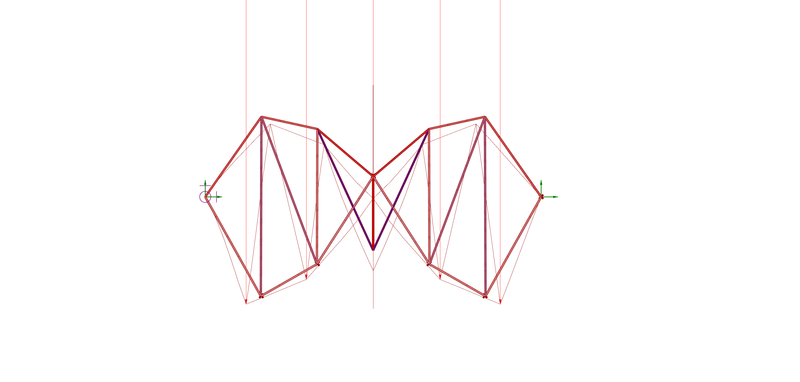
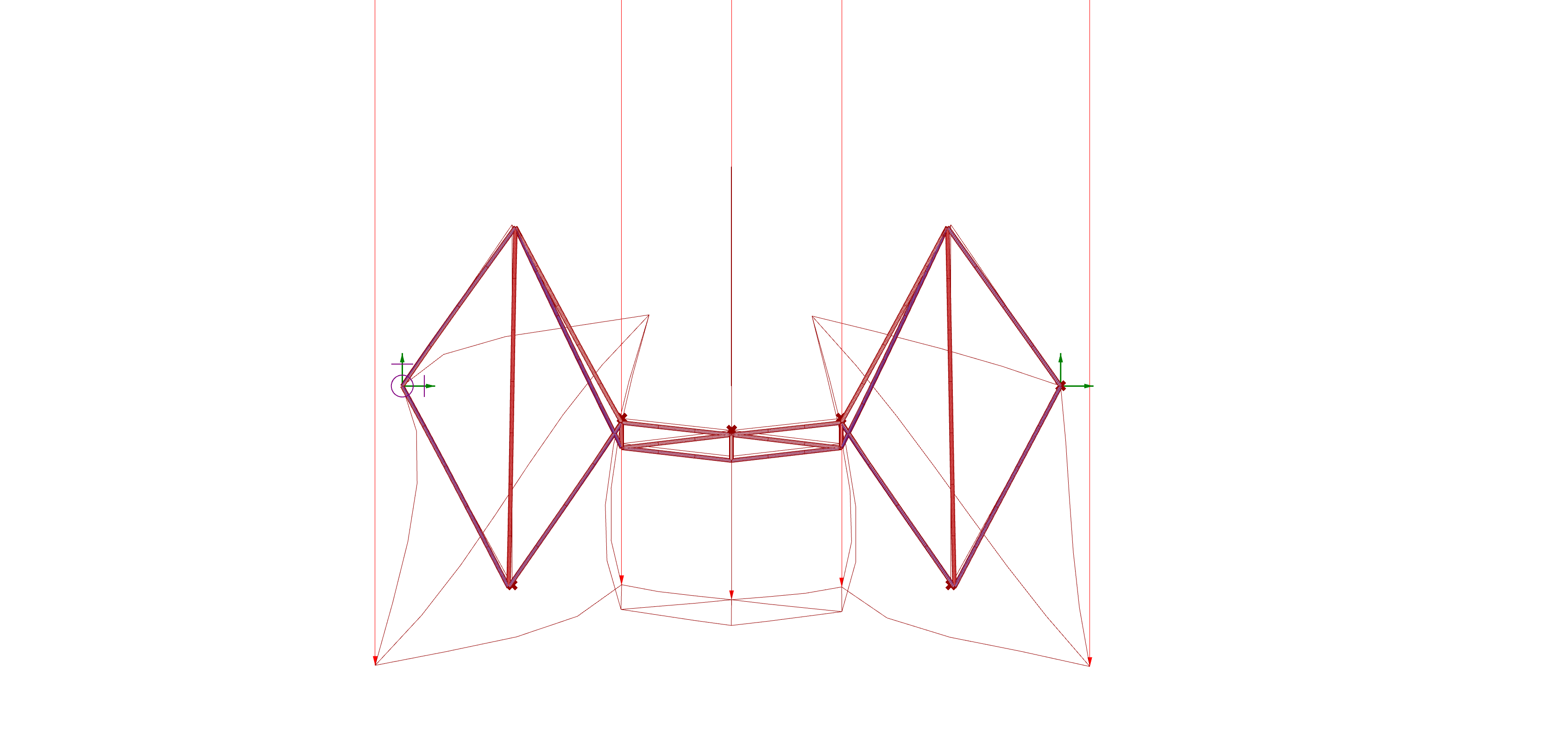
As a first step, we were asked to design in a parametrical way inside the GH gui a 2D truss structure, with a symmetry shape in the center bar but with different supports. One is a pin, able to deflect in rotation and the ohter one can be moved in the x axis. This led us to have a system with 6DOF which are the nodes of the bars. Each bar has a range of +- 3m in the y axis. 20kN loads will be applied in the lower nodes
Using Karamba, I have applied a cross-section of 7cm of diameter steel round tubes with a thickness of 1cm. We have calculated the volume load of the structure, as usual and we are ready to start optimizing!
a_ Optimizing with 6 variables
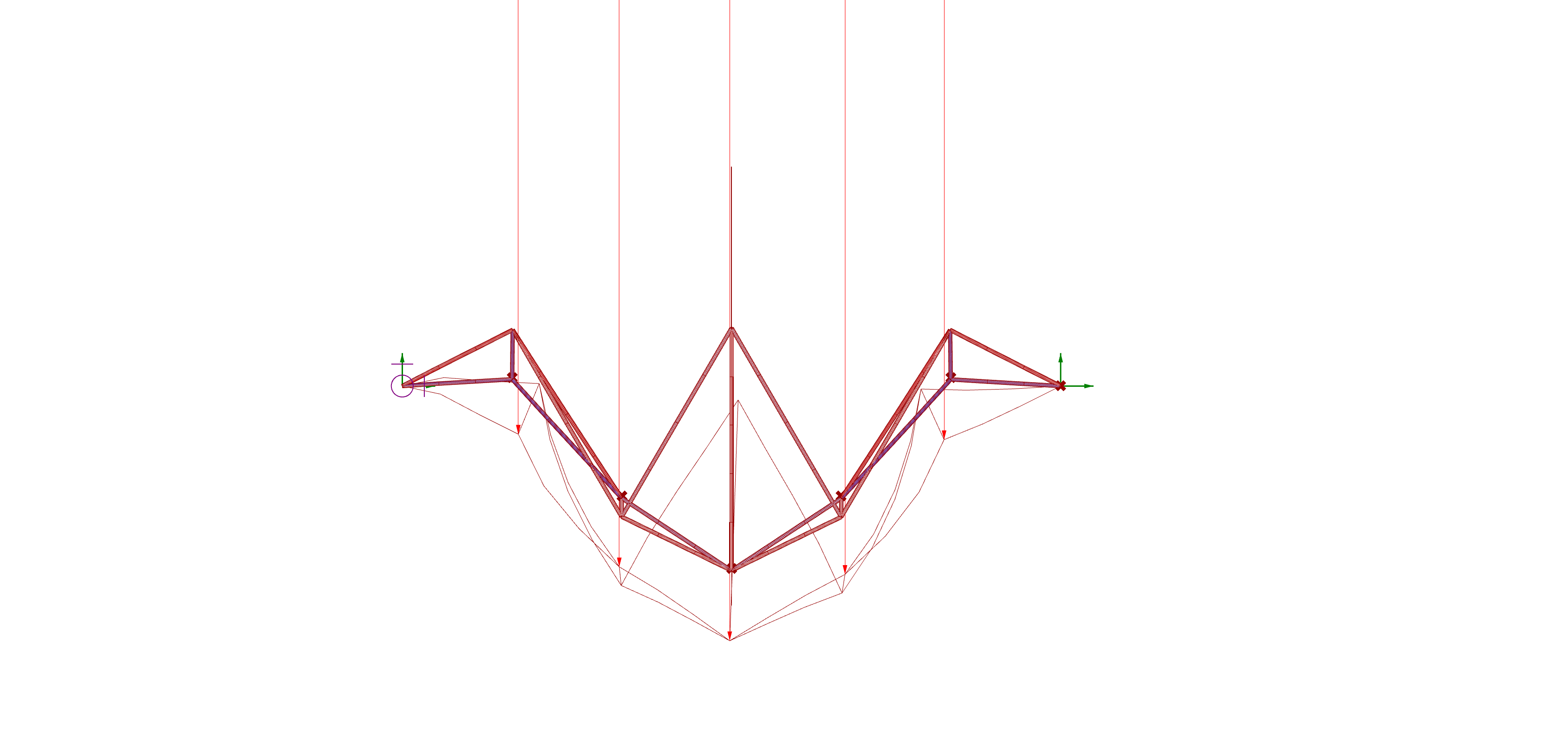
As a first step, seem difficult to optimize a 6DOF design space and be able to converge in a reasonable quantity of time. I linked goat to the DOf problem and after clicking for the first itme, I had to increase 30 second each iteration untill I reached a success. My optimization took finally 2 minits 30 seconds, but I reached a reasonable shape with a nice value of force per length.
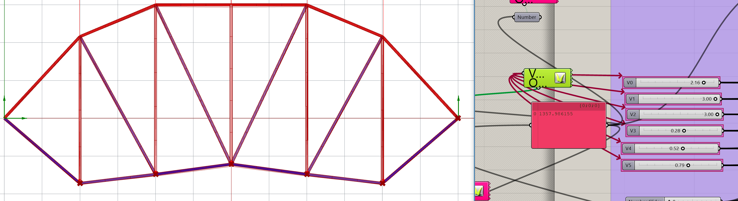
After the optimization in goat finished, I tried to modify the values of the sliders to improve the result and I couldnt. It makes sense due to I waited 3 minutes to conclude the optimization. I could improve the result if my goat optimization finished due to the maximun run time was used and the best result was not completed.
b_ Sampler and Capture
After some adaptation to use properly those tools, I was able to plot random data from my design space with the followinf results. Those are the 20 images obtained
The CSV data of the 20 parameters can be downloaded in the files to download at the beggining of this page.
After this point, I was ready to run my 2k cases. I knwew it was gonna be tricky to my computer and yes, it was.
You can download the CSV file of the 2k elements
c_ Playing with the 2k elements
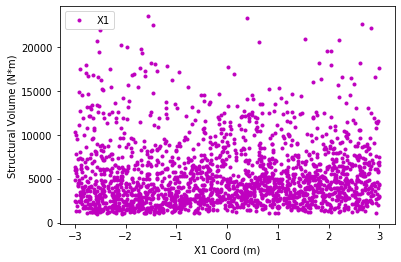
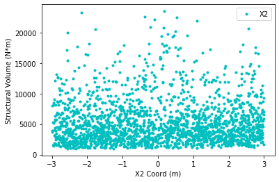
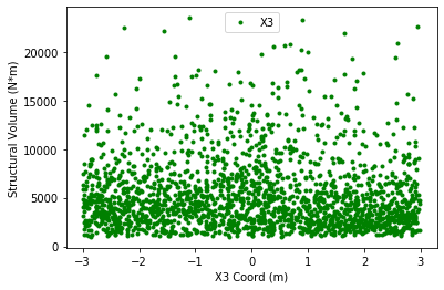
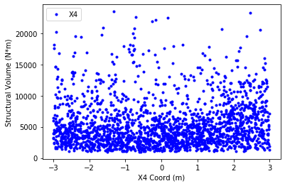
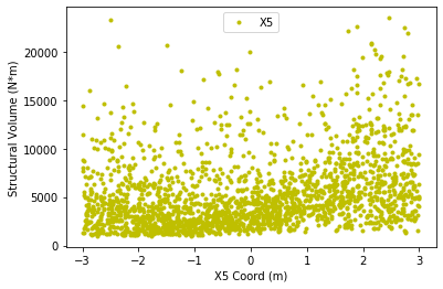
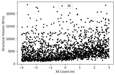
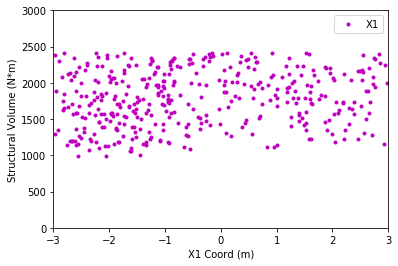
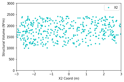
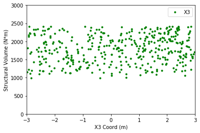
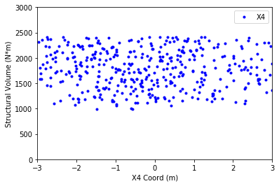
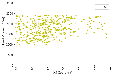
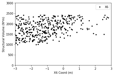
As I didn't read the full point, my first scatterplots were without filtering data. But I consider interesting to visualize filtered data vs non filtered data to see how the range of the y axis converge into interesting objective finction values.
To plot the data I used pandas and numpy in a python script importing, first the non filtered data.
Then, as I finished to read that I should data, I filtered only the 400 best optimization goals and those 400 samples looks like this
d_ Trying PCA in python, failing and doing it in Matlab
I really tried to succeed my PCA analysis in python but the output results has been that confising in range that I finally asked for help to my final project mate, Heather Nelson for some help in th PCA analysis. The result of the PCA analysis in Matlab was a matrix 3 x 6. Definitely, nest thursday I will go to the TA hours due to I am so interesting in this technique of dimentionally reduction and ask to understand better the python script.
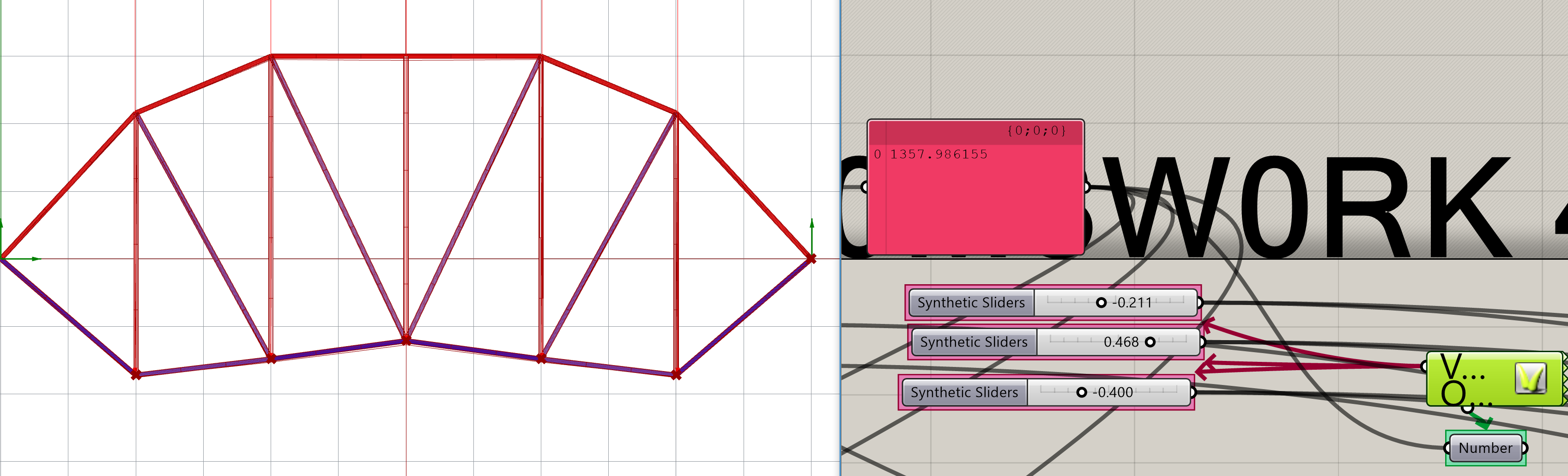
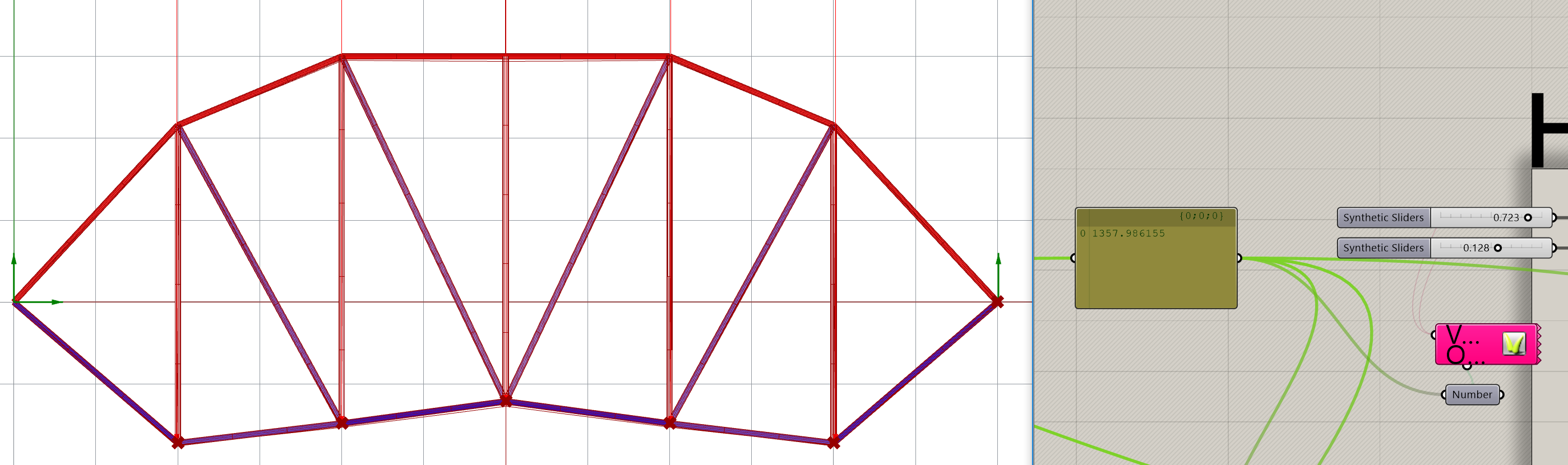
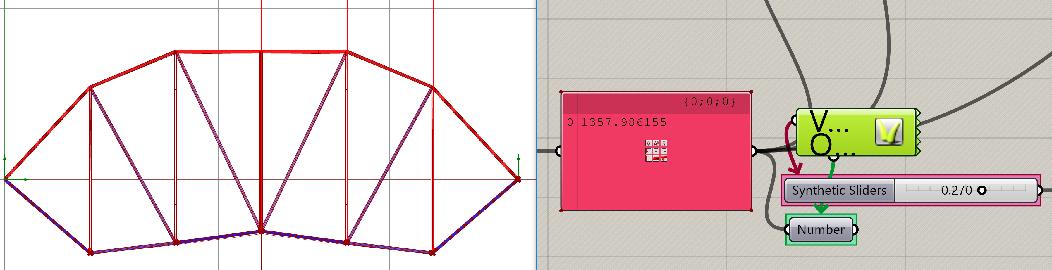
You can download the matrix of PCA in the download section. Also, It was time to generate synthetic variables. To be fair, the first slider were the one that modifies most drastically the optimization.
It is so beautifull how the potentiometers change the structure, and I could reach a really similar form only uning the first slider. This can be interesting to do herarchical optimiations in steps!
e_ Optimizing with Synthetic variables
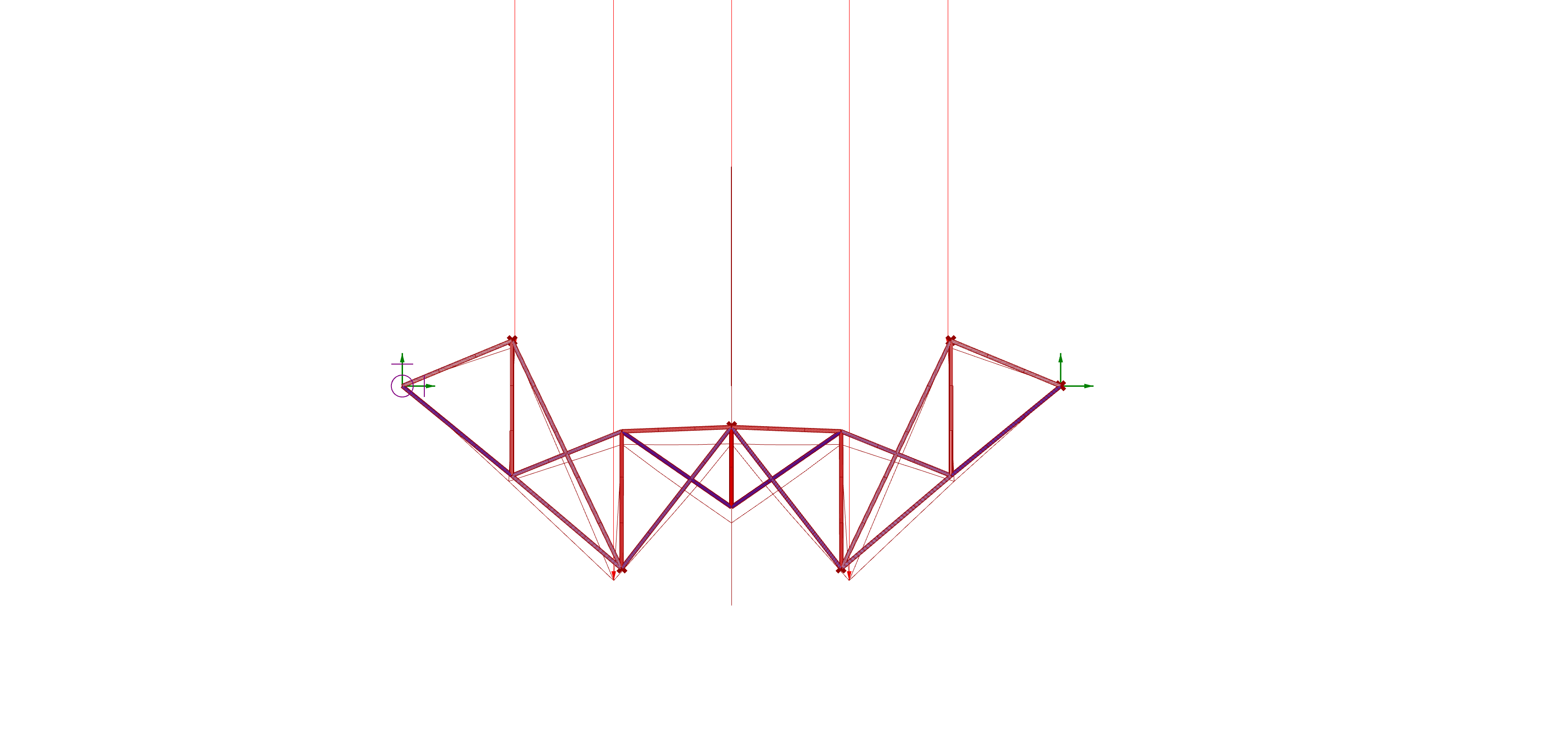
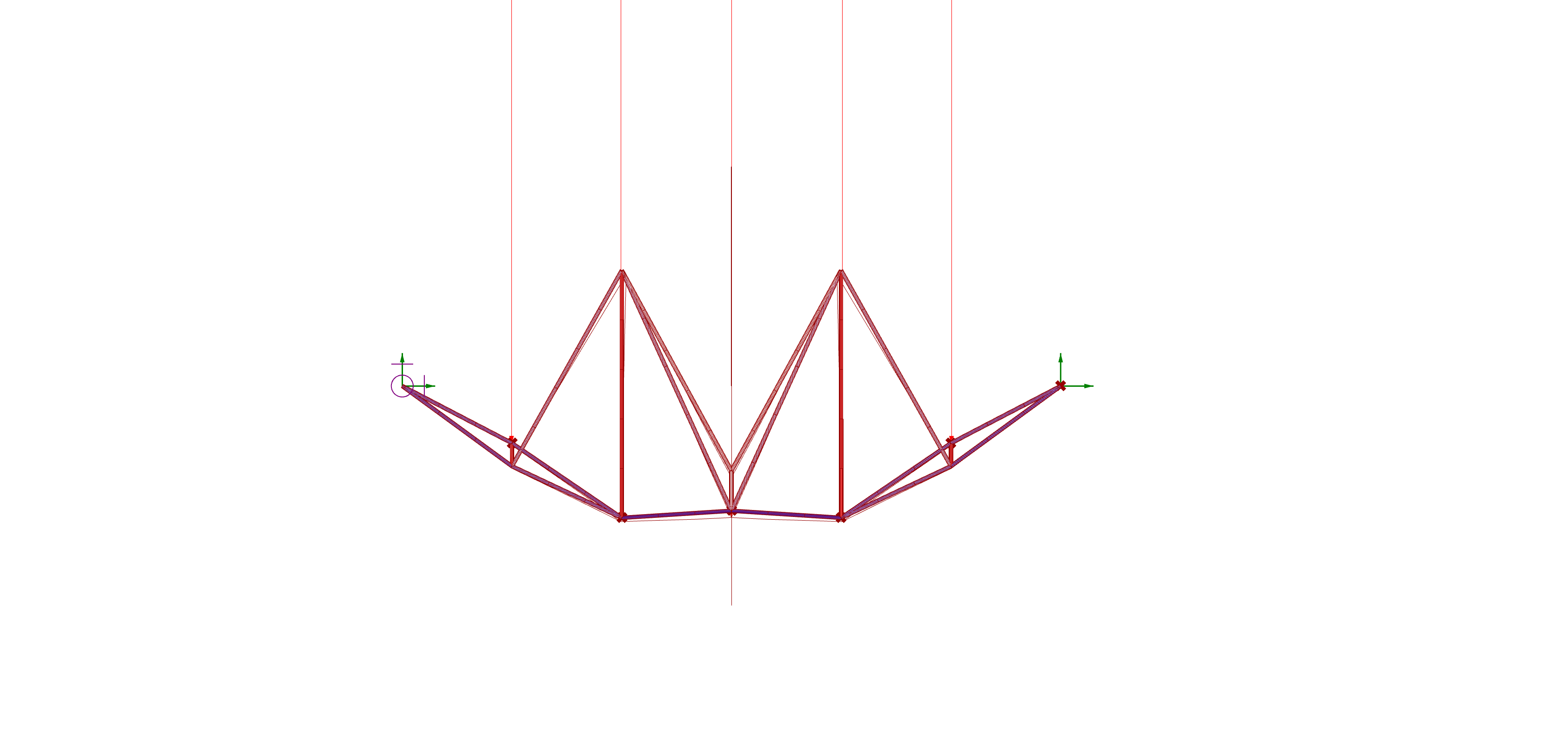
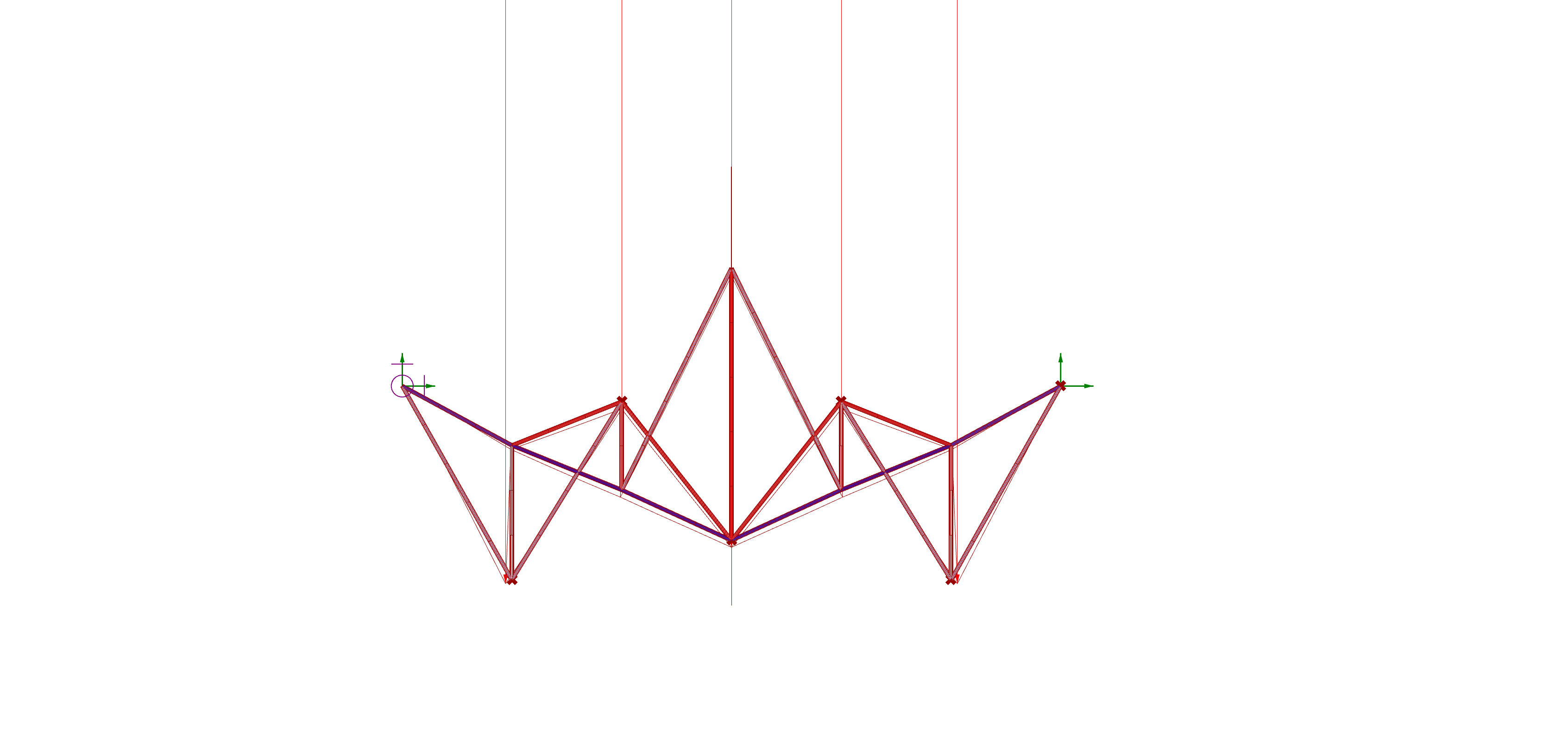
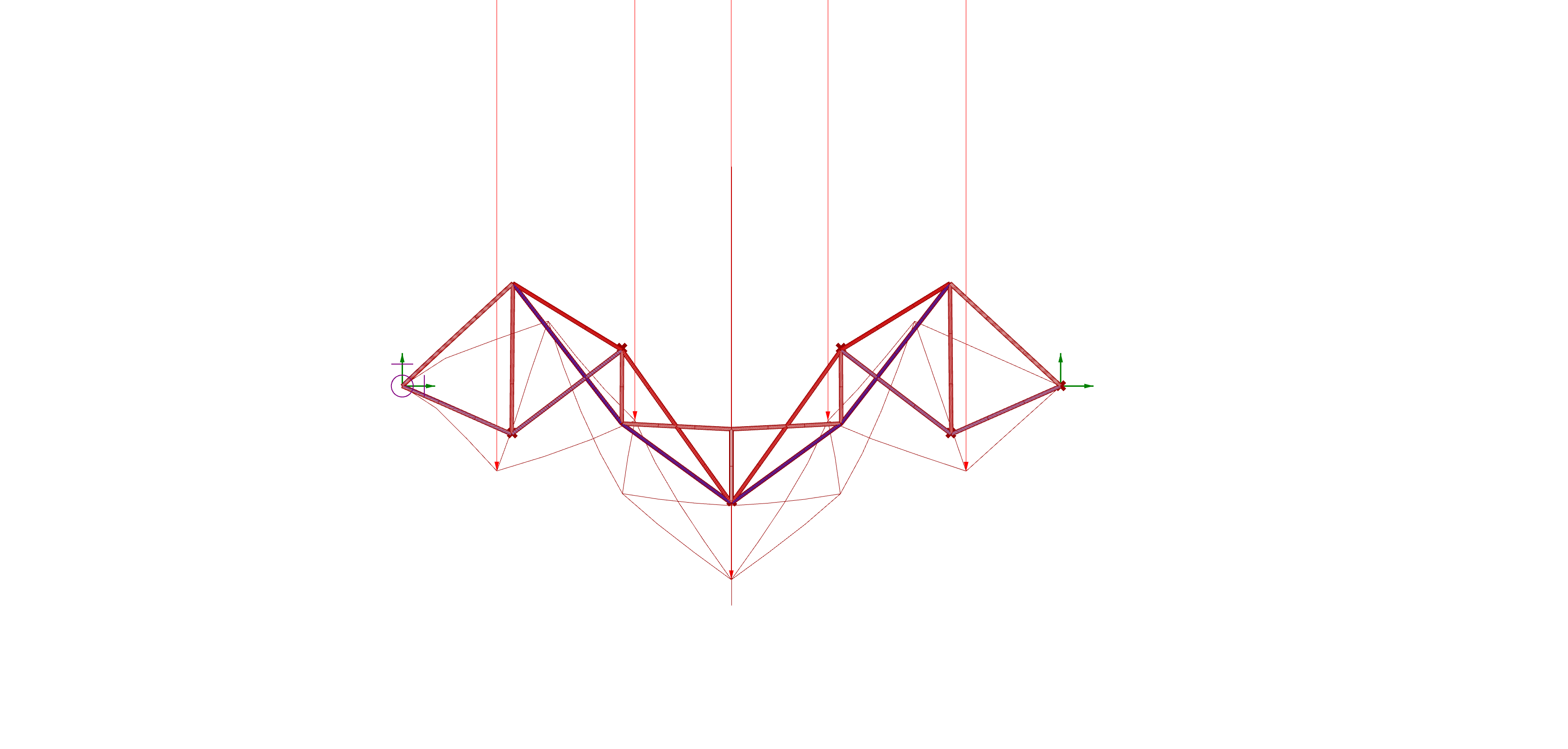
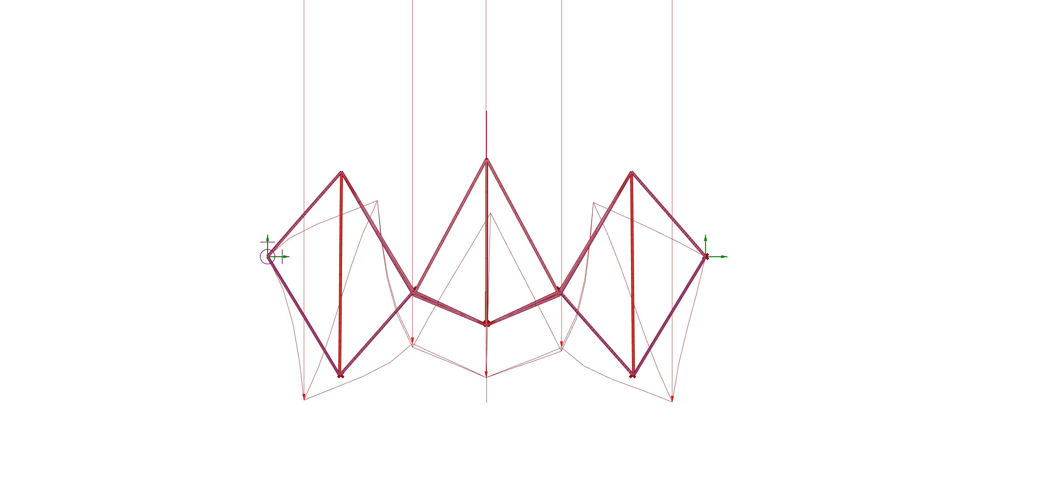
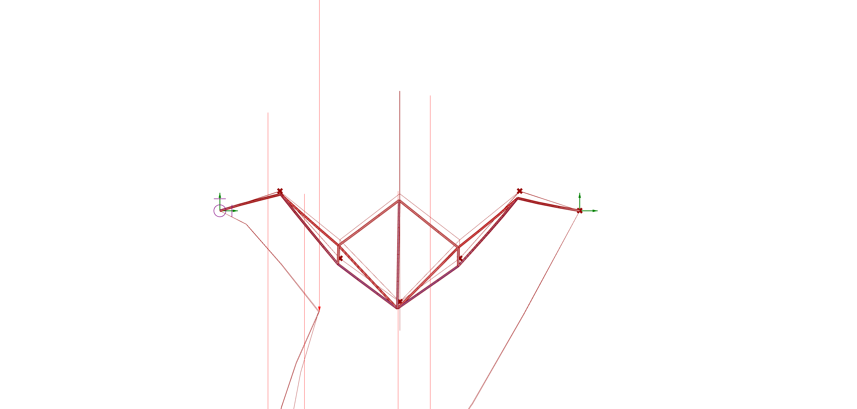
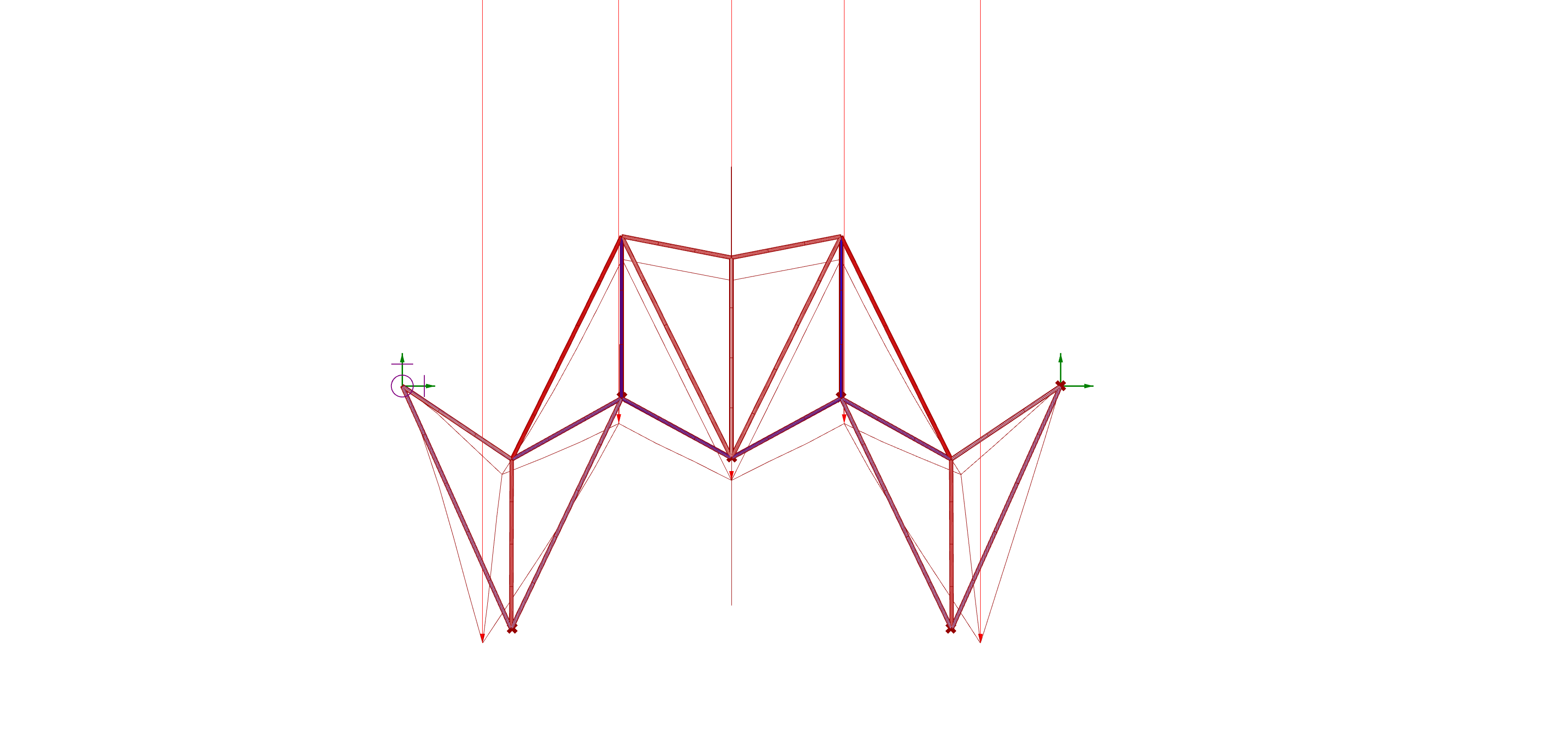
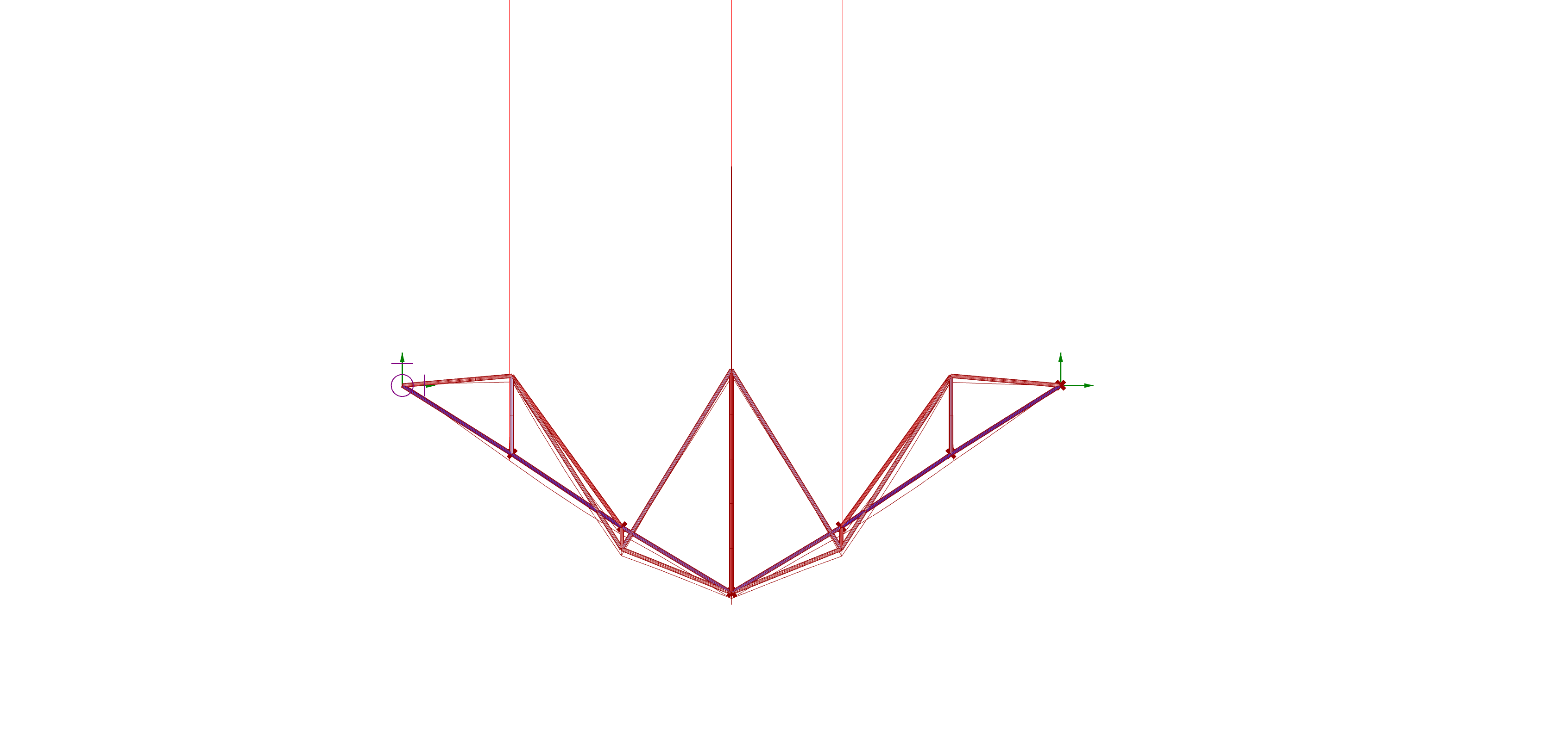
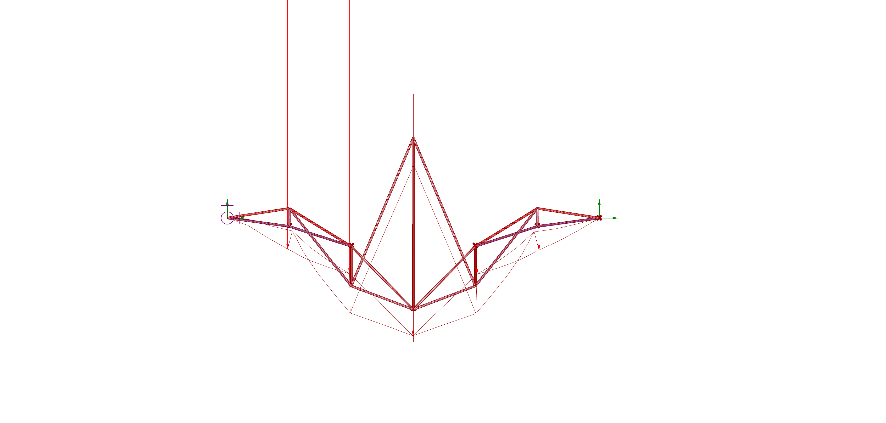
Now, I implementer three goat optimizations to each group of synthetic variables. The optimization of each case can be seen in the following three images.
3 syn var
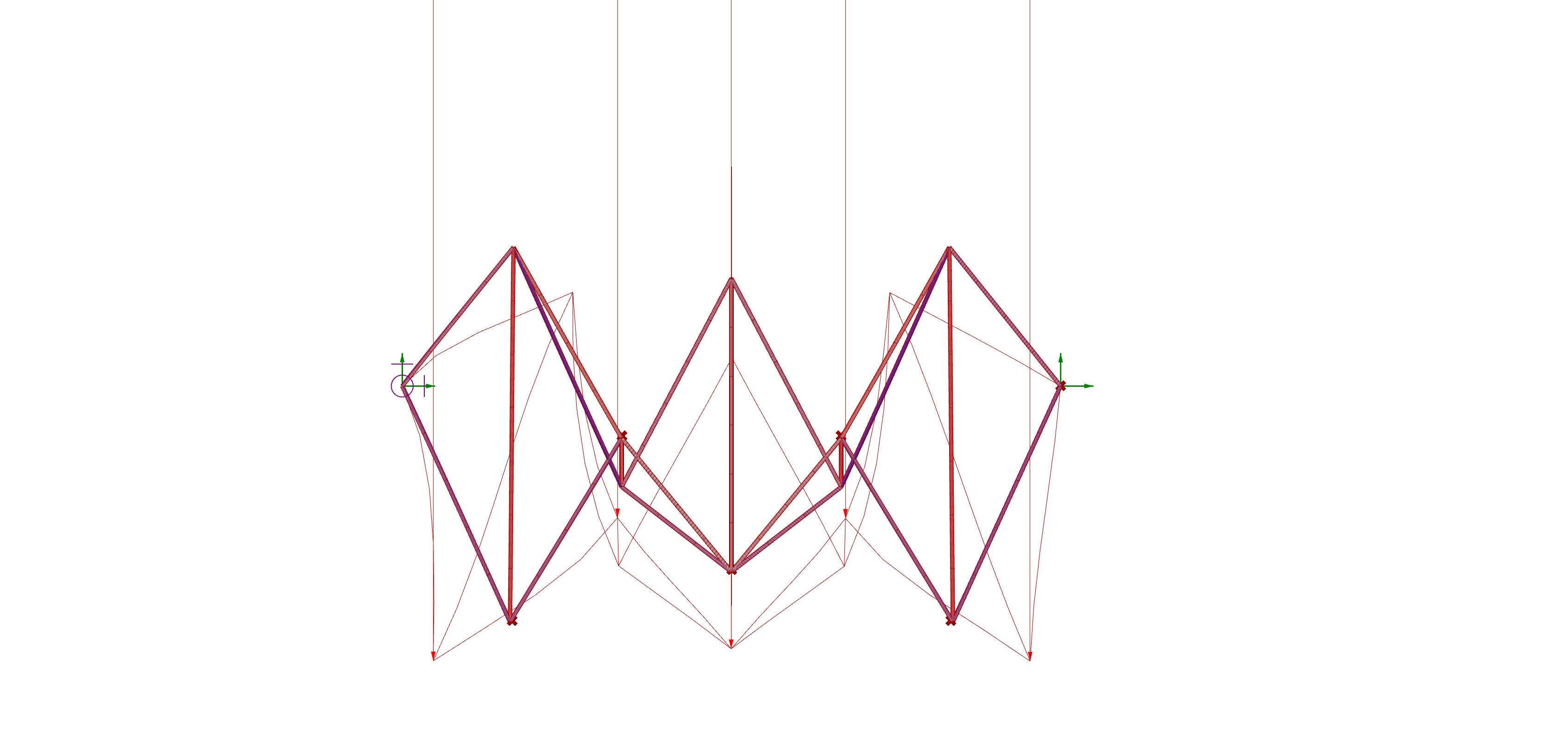
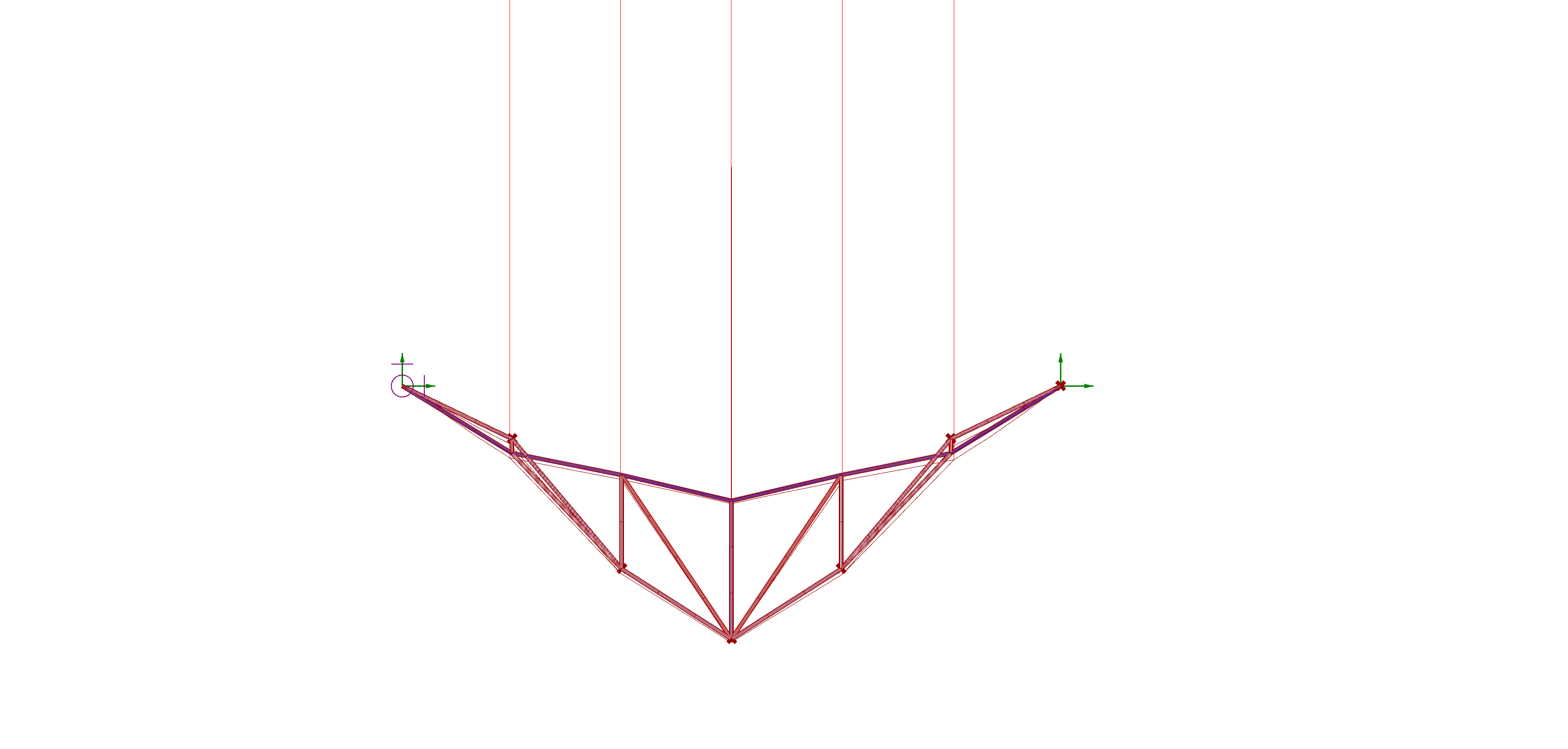
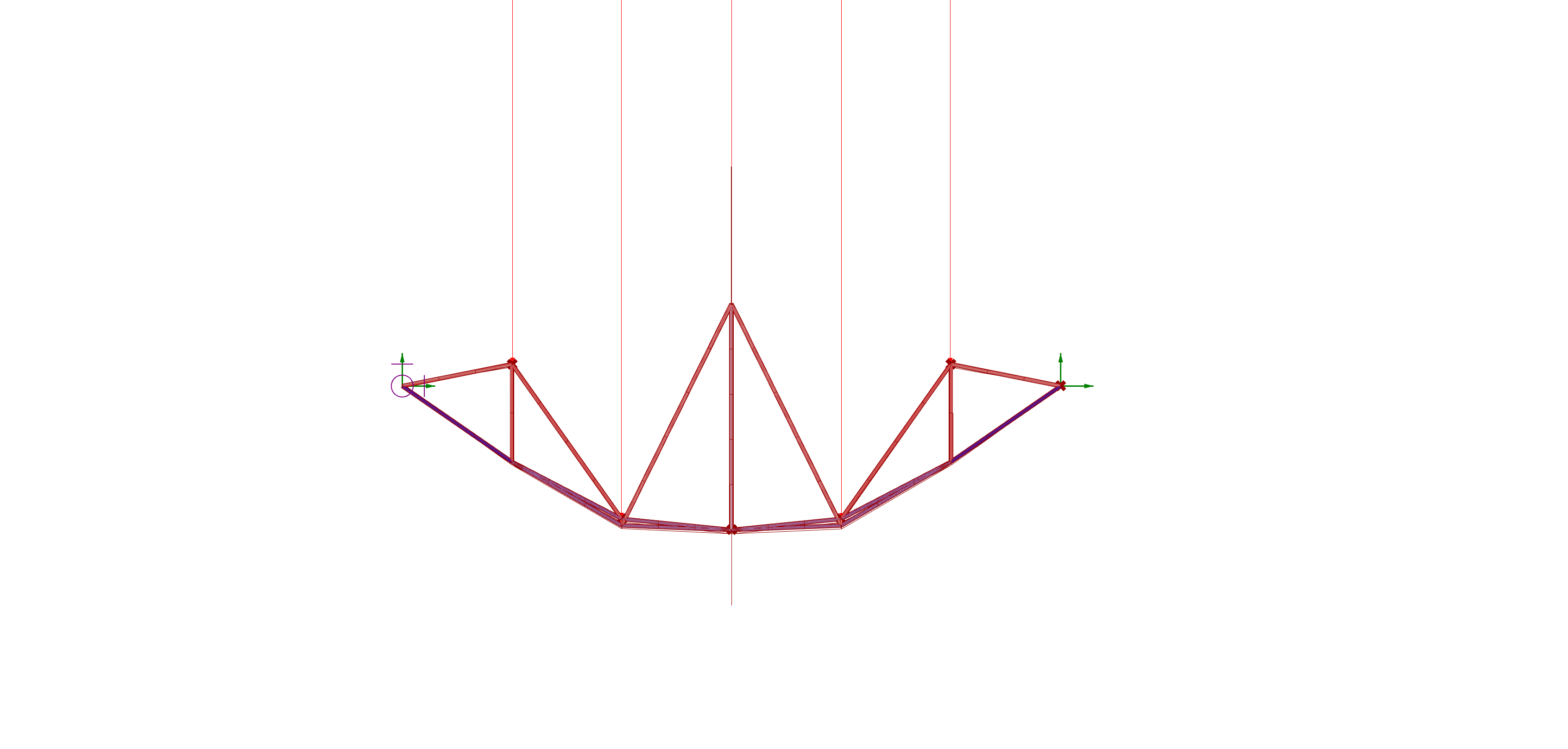
2 syn var
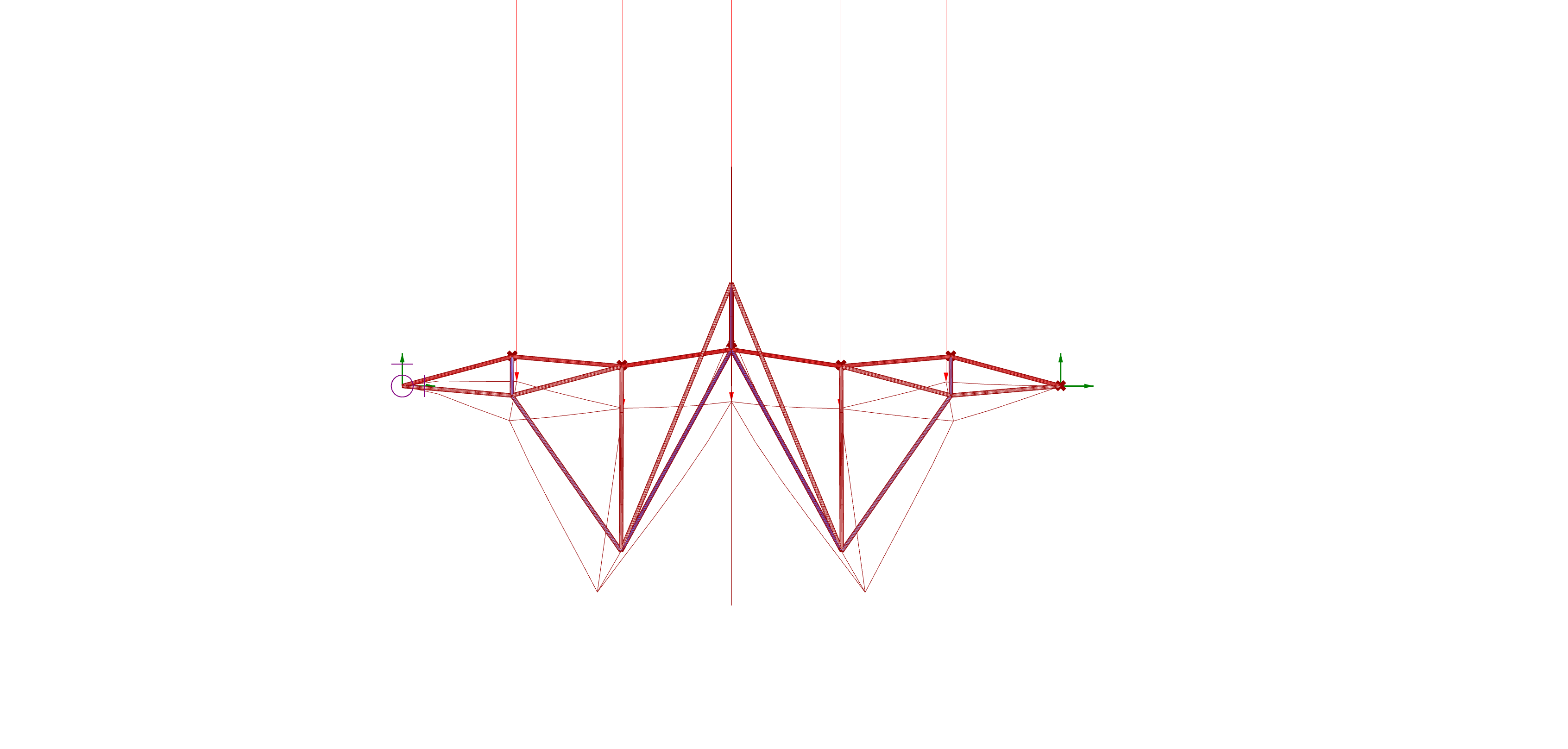
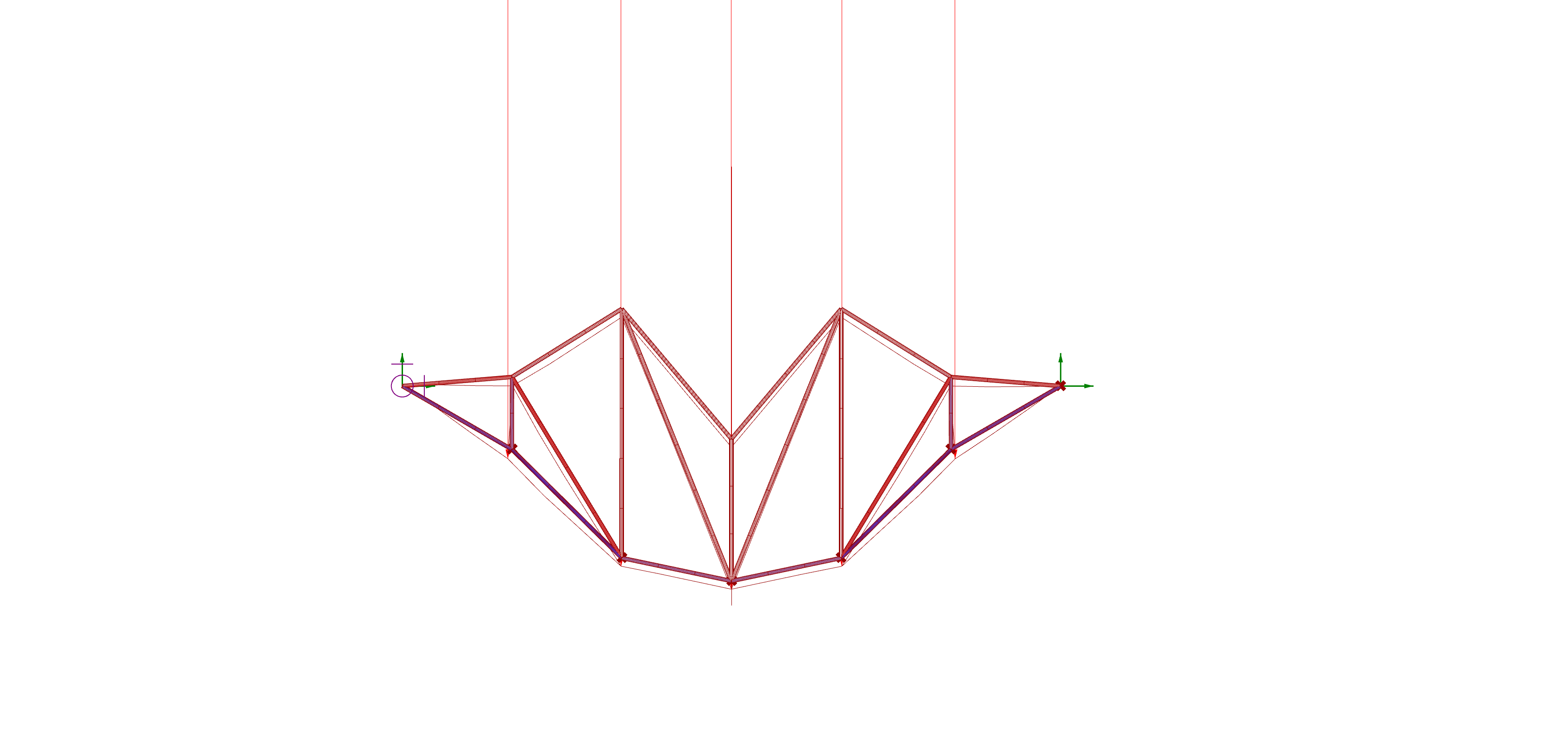
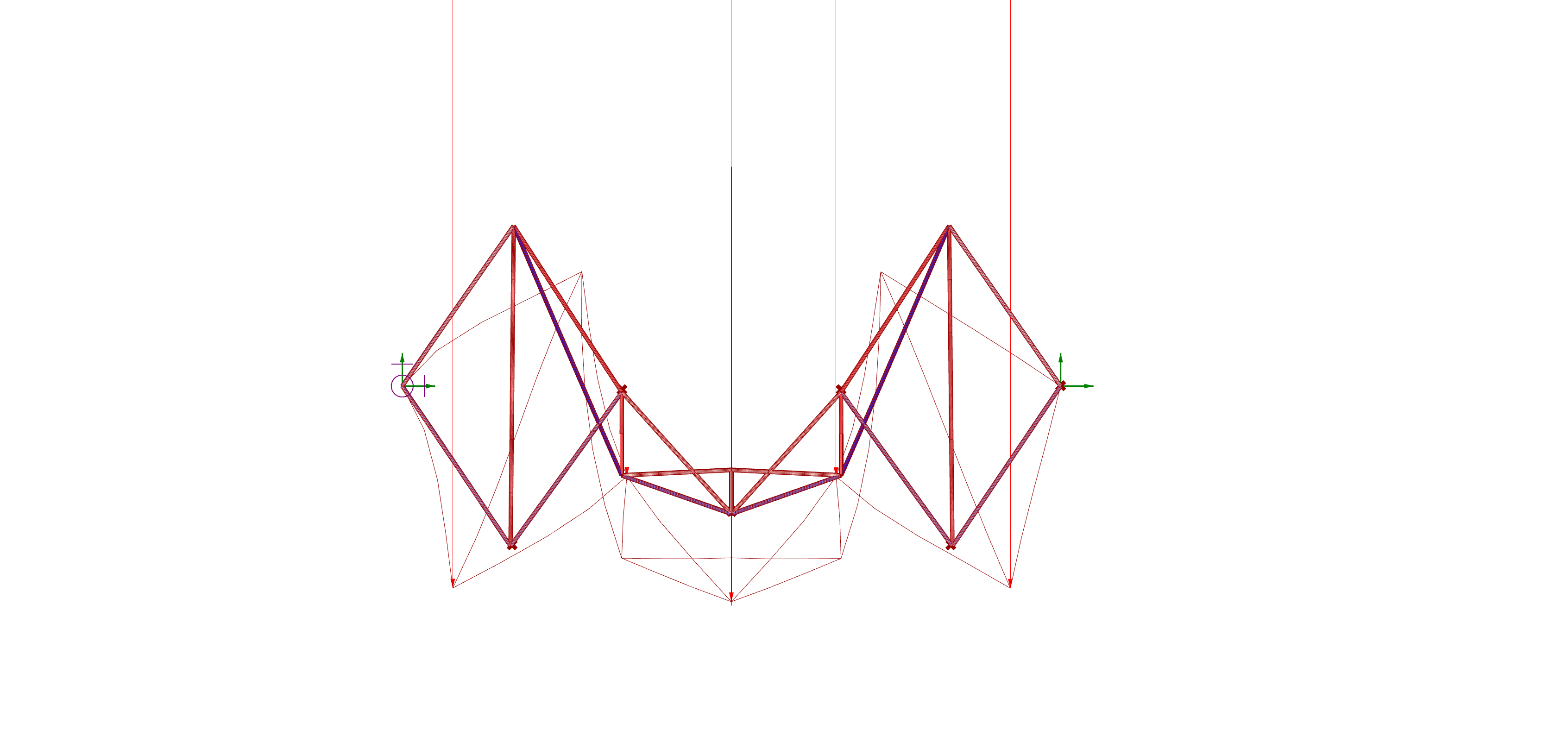
1syn var
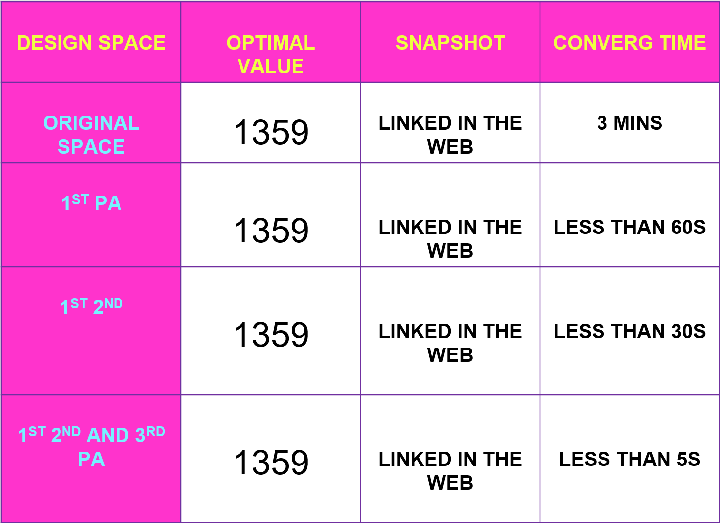
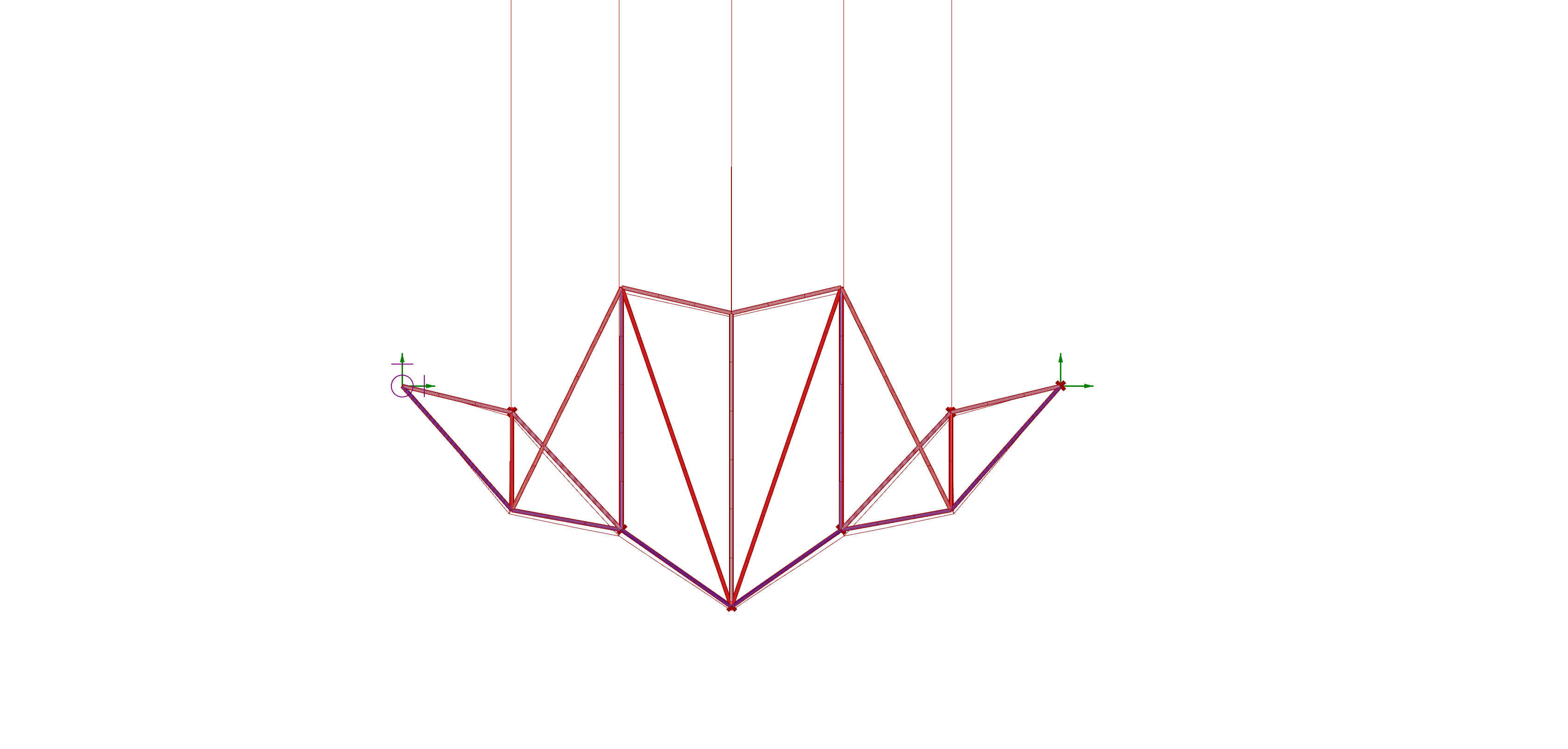
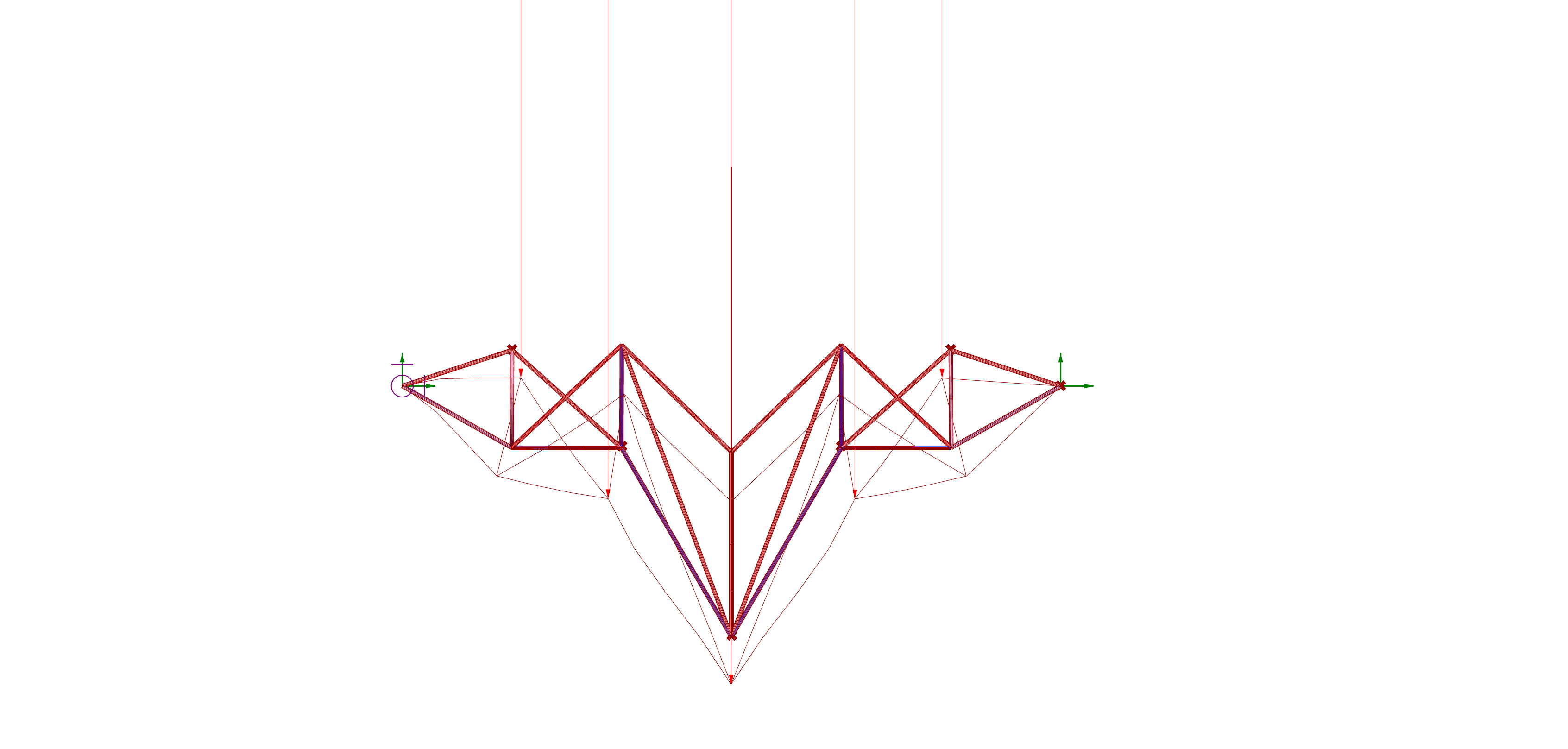
It can be seen that in all cases the optimization has been reached and the value of the result are the same. The only thing that drastically has change is the time to converge.
f_ Filling the table